Calculating summary statistics, probabilities and confidence intervals

Introduction

Aims

You will practice calculating and choosing summary statistics, quantiles and confidence intervals.

Learning Outcomes

By actively following the lecture and practical and carrying out the independent study the successful student will be able to:

• Explain the properties of ‘normal distributions’ and their use in statistics (MLO 1 and 2)
• Define, select and calculate with R probabilities, quantiles and confidence intervals (MLO 3 and 4)

Philosophy

Workshops are not a test. It is expected that you often don’t know how to start, make a lot of mistakes and need help. Do not be put off and don’t let what you can not do interfere with what you can do. You will benefit from collaborating with others and/or discussing your results.

The lectures and the workshops are closely integrated and it is expected that you are familar with the lecture content before the workshop. You need not understand every detail as the workshop should build and consolidate your understanding. You may wish to refer to the slides as you work through the workshop schedule.

Slides

Calculating summary statistics, probabilities and confidence intervals: pdf (recommended) / pptx

Artwork by Allison Horst

Getting started

Start RStudio from the Start menu.

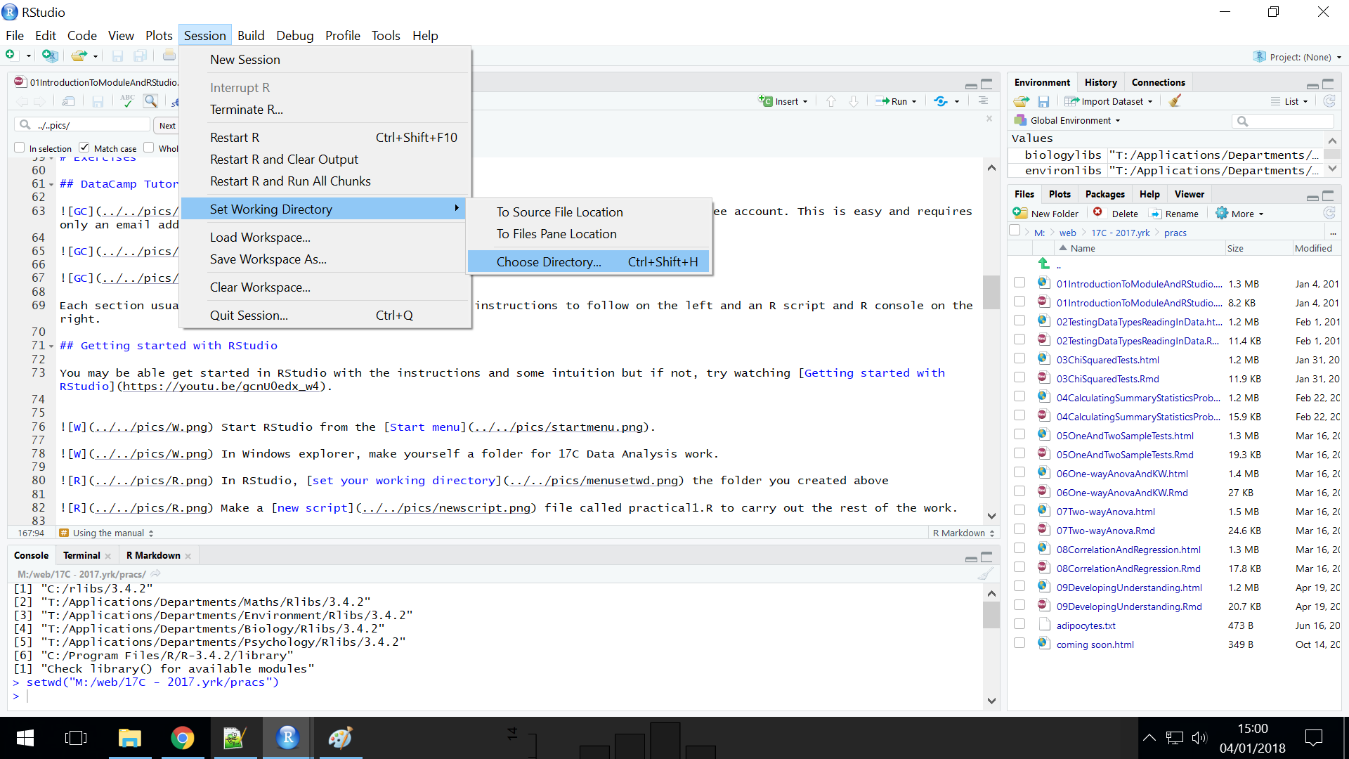
In RStudio, set your working directory to the folder you created previously for your 17C Data Analysis work.

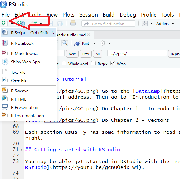
Make a new script file called practical4.R to carry out the rest of the work.

Exercises

Distributions: the R functions

For any distribution, two very useful quantities can be calculated:
* the Distribution Function, which gives the probability that a variable takes a particular value or less.
* the Quantile function which is the inverse of the Distribution function, i.e., it returns the value (‘quantile’) for a given probability.

The functions are names with a letter p or q preceding the distribution name. Below are some examples:

	Probability	Quantile
Binomial distribution	pbinom()	qbinom()
Normal distribution	pnorm()	qnorm()
t distribution	pt()	qt()

Calculating Probabilities for single value

Using pnorm()

Look up pnorm() in the manual using ?pnorm

You give it a values for which you want a probability and by default it gives you the probability of getting that value or less from a normal distribution with a mean of 0 and a standard devation of 1. If you want the probability of a vlaue from a different normal distribution you need to set the mean and standard deviation appropriately.

For example, I.Q. in the U.K. population is normally distributed with a mean of 100 and a standard deviation of 15. We can use pnorm() to calculate probabilities associated with having a particular range of IQs.

We can use the values of mean = 100 and standard deviation = 15 in pnorm() to work out the probability of having an I.Q. of 115 or less.

First, create variables for the parameter values - this is considered good practice.

# create variables for the parameter values
m <- 100
sd <- 15

Now pass those variables to the pnorm() function along with the value for which we want a probability:

# Now use pnorm()
pnorm(115, m, sd)

## [1] 0.8413447

Look at the manual page. Because the default is lower.tail = TRUE, we get the probability we want, P[IQ < 115]

I recommend sketching the distribution and shading the area you want to work out what arguments you want to give the function.

Determine the probability of having an IQ of 115 OR MORE? Do a sketch first.

Determine the probability of having an IQ between 85 and 115? Do a sketch first.

Is this what you expect?

What is 1.96 * the standard deviation

What is the probability of having an IQ between -1.96 standard deviations and +1.96 standard deviations? Is this what you expect?

Using qnorm()

We can use qnorm() to find the IQ associated with a particular probability.

We will again use the values of mean = 100 and standard deviation = 15 in qnorm() to work out what I.Q. value 0.2 (20%) of people fall below. Make sure you relate the manual information to the command.

To find the I.Q. value that 20% people fall below:

 qnorm(0.2, m, sd)

## [1] 87.37568

20% people have an IQ less than 87.4

What I.Q. value are 0.025 (2.5%) of people below?

In what range do 99% of the population fall? Note that 99% means 1% (0.01) in both tails so 0.5% (0.005) in each tail. The figure may help you.

Calculating Probabilities for samples

The only difference in using pnorm() and qnorm() for samples is in what we give as the sd argument. Since we are now thinking about the distribution of the sample means, we need to use the standard error.

We used mean = 100 and standard deviation = 15 in pnorm() to work out the probability of an individual having an I.Q. of 115 or less.

We can use a similar approach to find the probability of getting a sample of n = 5 having a mean I.Q. of 115 or less The only difference is that we use the standard error instead of the standard deviation.

First, calculate the standard error:

n <- 5
se <- 15 / sqrt(n)

Now the probability of getting a sample mean of 115 or less from that distribution:

pnorm(115, m, se)

## [1] 0.9873263

There’s a 0.9873 probability that a sample of 5 people will have a mean of 115 or less. Thus there is a probability of just 0.0127 that a sample of n = 5 will have a mean above 115. This is quite unlikely and we might suspect this group was not sampled from the general population.

What is the probability of sample of size 10 having a mean of 105 or more?

Confidence intervals (large samples)

The data in beewing.txt are left wing widths of 100 honey bees (mm). The confidence interval for large samples is given by: \(\bar{x} \pm 1.96 \times s.e.\))

Where 1.96 is the quantile for 95% confidence.

You may need to refer to previous practicals to remind yourself how to carry out some of the following steps.

Save a copy of the file. I saved mine to my ‘data’ directory

Read in the data and check the structure of the resulting dataframe

Rename the column to ‘wing’

Calculate and assign to variables: the mean, standard deviation and standard error

To calculate the 95% confidence interval we need to look up quantile (multiplier) using qnorm()

q <- qnorm(0.975)

Now we can use it in our confidence interval calculation

(lcl <- m - q * se)

## [1] 4.473176

(ucl <- m + q * se)

## [1] 4.626824

Between what values would you be 99% confident of the population mean being?

Confidence intervals (small samples)

The confidence interval for small samples is given by: \(\bar{x} \pm \sf t_{[d.f]} \times s.e.\)

The fatty acid Docosahexaenoic acid (DHA) is a major component of membrane phospholipids in nerve cells and deficiency leads to many behavioural and functional deficits. The cross sectional area of neurons in the CA 1 region of the hippocampus of normal rats is 155 \(\mu m^2\). A DHA deficient diet was fed to 8 animals and the cross sectional area (csa) of neurons is given in neuron.txt

Save a copy of the file. I saved mine to my ‘data’ directory

Read in the data and check the structure of the resulting dataframe

Assign the mean to m

Calculate and assign the standard error to se

To work out the confidence interval for our sample mean we need to use the t distribution because it is a small sample. This means we need to determine the degrees of freedom (the number in the sample minus one).

We can assign this to a variable using:

df <- length(neur$csa) - 1; df

## [1] 7

The t value is found by:

t <- qt(0.975, df = df); t

## [1] 2.364624

And the confidence interval by:

round(m + t * se, 2)

## [1] 151.95

round(m - t * se, 2)

## [1] 132.75

Given the upper and lower confidence values for the estimate of the population mean, what do you think about the effect of the DHA deficient diet?

Independent study

You need to carry out this work before the next practical.

Reading

An introduction to the normal distribution from the Teacups, giraffes and statistics book (the whole online book is listed in the Additional Resources folder on the VLE).

Confidence interval

Adiponectin is exclusively secreted from adipose tissue and modulates a number of metabolic processes. Nicotinic acid can affect adiponectin secretion. 3T3-L1 adipocytes were treated with nicotinic acid or with a control treatment and adiponectin concentration (pg/mL) measured. The data are in adipocytes.txt. Each row represents an independent sample of adipocytes and the first column gives the concentration adiponectin and the second column indicates whether they were treated with nicotinic acid or not. Estimate the mean Adiponectin concentration in each group - this means calculate the sample mean and construct a confidence interval around it for each group. Hint: you will find ‘tapply()’ which was in a previous practical useful.

Probability of misdiagnosis

Healthy people have Thyroid Stimulating Hormone (TSH) levels of (mean \(\pm\) s.d) 3 \(\pm\) 2.8 units per mL of blood, those experiencing hypothyroidism have elevated TSH. Individuals with TSH 6 units per mL or higher are treated for hypothyroidism. What is the probability of being misdiagnosed with hypothyroidism?

Geting a bit oveRwhelmed?

Try Chapter 3 Getting started with R of Danielle Navarro’s book.

The Code files

These contain answers and code even though they do not appear on the webpage itself.

Rmd file The Rmd file is the file I use to compile the practical. Rmd stands for R markdown allow R code and ordinary text to be inter weaved to produce well-formatted reports including webpages.

Plain script file This is plain script (.R) version of the practical

Script example

This is an example of a well formatted analysis script

Script example

Objectives from previous sessions

Introduction to module and RStudio

• to explain why we need statistical tests and the logic of hypothesis testing (MLO 1)
• use the R command line as a calculator and to assign variables (MLO 3)
• create and use the basic data types in R (MLO 3)
• find their way around the RStudio windows (MLO 3)
• create, use and save a script file to run r commands (MLO 3)
• search and understand manual pages (MLO 3)

Testing, Data types and reading in data

• to able to explain what response and explanatory variables are, distinguish between data types and describe how these impact choice of test (MLO 1 and 2)
• demonstrate the process of hypothesis testing with an example and evaluate potential inferences (MLO 1 and 2)
• read in data in to RStudio, create simple summaries and plots using manual pages where necessary (MLO 3)
• create neat reports in Word which include text and figures (MLO 4)

Goodness of Fit and Contingency chi-squared tests

• recognise when to use chi-squared Goodness of Fit and Contingency tests (MLO 2)
• be able to carry out, interpret and report scientifically both types in R (MLO 3 and 4)